
Fichier:Bloop locations.png
Taille de cet aperçu : 600 × 600 pixels. Autres résolutions : 240 × 240 pixels | 480 × 480 pixels | 768 × 768 pixels | 1 024 × 1 024 pixels | 2 048 × 2 048 pixels | 3 000 × 3 000 pixels.
Fichier d’origine (3 000 × 3 000 pixels, taille du fichier : 7,74 Mio, type MIME : image/png)
Ce fichier et sa description proviennent de Wikimedia Commons.
Description
| Description |
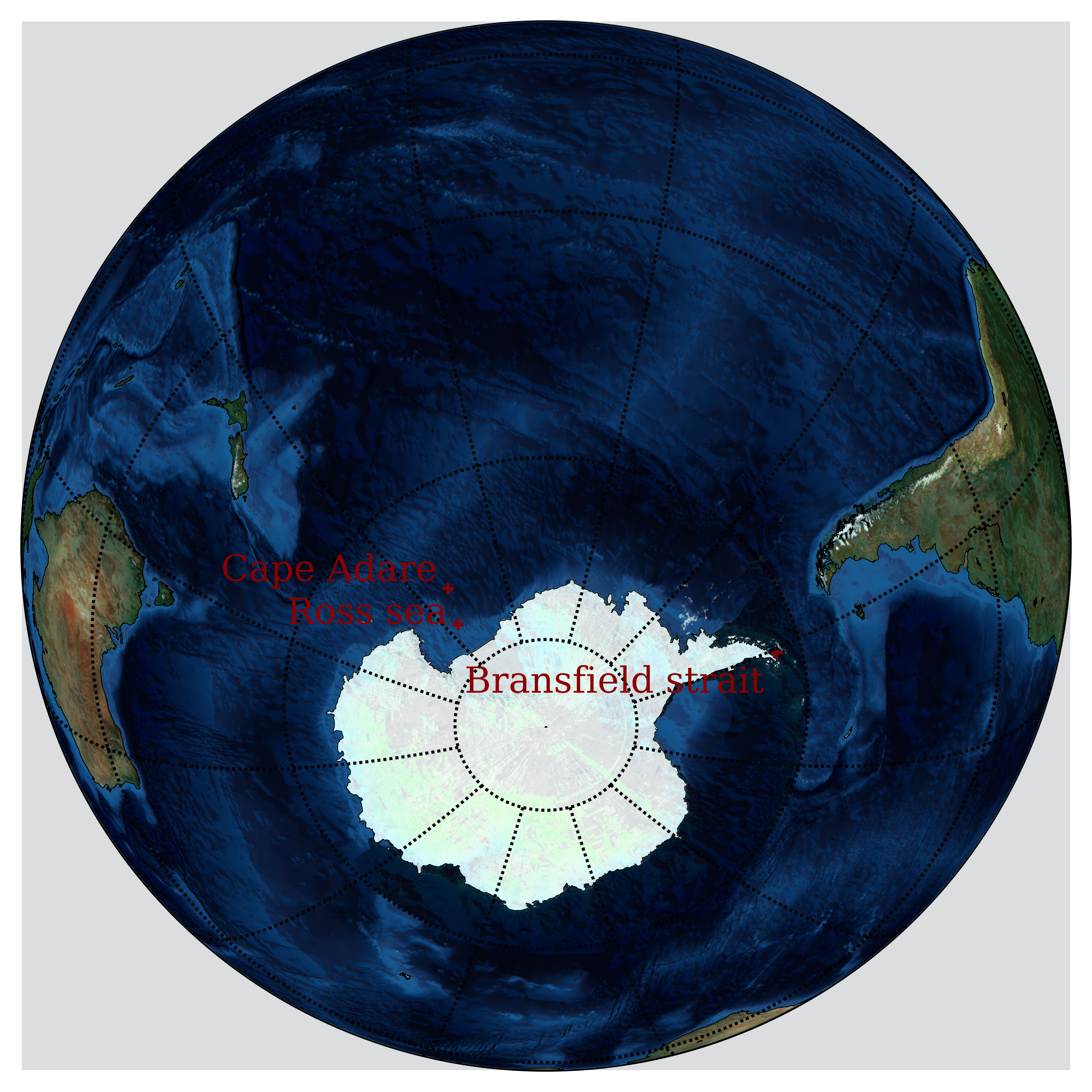
English: Possible locations of the Bloop, an ultra-low frequency and extremely powerful underwater sound detected by the U.S. National Oceanic and Atmospheric Administration (NOAA) in 1997. |
| Date | |
| Source | Travail personnel |
| Auteur | Nojhan |
| PNG information | Cette PNG image matricielle a été créée avec Python |
Source code
This image has been generated by the following source code in Python:
Python code
| source code |
|---|
print "import modules...",
import sys
sys.stdout.flush()
import pickle
from mpl_toolkits.basemap import Basemap, shiftgrid, cm
import matplotlib
import matplotlib.pyplot as plt
import numpy as np
from netCDF4 import Dataset
print "ok"

# Lovecraft: 47:9'S 126:43'W
# lovecraft_lat = -47.9
# lovecraft_lon = -126.43

# August Derleth: 49:51'S 128:34'W
# derleth_lat = -49.51
# derleth_lon = -128.34

# Nemo point: 48:52.6'S 123:23.6'W
# nemo_lat = -48.526
# nemo_lon = -123.236

# The Bloop:
bransfield_strait_lat=-63
bransfield_strait_lon=-59
ross_sea_lat = -75
ross_sea_lon = -175
cape_adare_lat = -71.17
cape_adare_lon = -170.14

mid_lat = np.mean((bransfield_strait_lat,ross_sea_lat,cape_adare_lat))
mid_lon = np.mean((bransfield_strait_lon,ross_sea_lon,cape_adare_lon))


# Not necessary, because the default projection is ortho,
# but can be useful if you want another one.
def equi(m, centerlon, centerlat, radius, *args, **kwargs):
    """
    Drawing circles of a given radius around any point on earth, given the current projection.
    http://www.geophysique.be/2011/02/20/matplotlib-basemap-tutorial-09-drawing-circles/
    """
    glon1 = centerlon
    glat1 = centerlat
    X = []
    Y = []
    for azimuth in range(0, 360):
        glon2, glat2, baz = shoot(glon1, glat1, azimuth, radius)
        X.append(glon2)
        Y.append(glat2)
    X.append(X[0])
    Y.append(Y[0])

    #m.plot(X,Y,**kwargs) #Should work, but doesn't...
    X,Y = m(X,Y)
    plt.plot(X,Y,**kwargs)


def shoot(lon, lat, azimuth, maxdist=None):
    """Shooter Function
    Plotting great circles with Basemap, but knowing only the longitude,
    latitude, the azimuth and a distance. Only the origin point is known.
    Original javascript on http://williams.best.vwh.net/gccalc.htm
    Translated to python by Thomas Lecocq :
    http://www.geophysique.be/2011/02/19/matplotlib-basemap-tutorial-08-shooting-great-circles/
    """
    glat1 = lat * np.pi / 180.
    glon1 = lon * np.pi / 180.
    s = maxdist / 1.852
    faz = azimuth * np.pi / 180.

    EPS= 0.00000000005
    if ((np.abs(np.cos(glat1))<EPS) and not (np.abs(np.sin(faz))<EPS)):
        alert("Only N-S courses are meaningful, starting at a pole!")

    a=6378.13/1.852
    f=1/298.257223563
    r = 1 - f
    tu = r * np.tan(glat1)
    sf = np.sin(faz)
    cf = np.cos(faz)
    if (cf==0):
        b=0.
    else:
        b=2. * np.arctan2 (tu, cf)

    cu = 1. / np.sqrt(1 + tu * tu)
    su = tu * cu
    sa = cu * sf
    c2a = 1 - sa * sa
    x = 1. + np.sqrt(1. + c2a * (1. / (r * r) - 1.))
    x = (x - 2.) / x
    c = 1. - x
    c = (x * x / 4. + 1.) / c
    d = (0.375 * x * x - 1.) * x
    tu = s / (r * a * c)
    y = tu
    c = y + 1
    while (np.abs (y - c) > EPS):

        sy = np.sin(y)
        cy = np.cos(y)
        cz = np.cos(b + y)
        e = 2. * cz * cz - 1.
        c = y
        x = e * cy
        y = e + e - 1.
        y = (((sy * sy * 4. - 3.) * y * cz * d / 6. + x) *
              d / 4. - cz) * sy * d + tu

    b = cu * cy * cf - su * sy
    c = r * np.sqrt(sa * sa + b * b)
    d = su * cy + cu * sy * cf
    glat2 = (np.arctan2(d, c) + np.pi) % (2*np.pi) - np.pi
    c = cu * cy - su * sy * cf
    x = np.arctan2(sy * sf, c)
    c = ((-3. * c2a + 4.) * f + 4.) * c2a * f / 16.
    d = ((e * cy * c + cz) * sy * c + y) * sa
    glon2 = ((glon1 + x - (1. - c) * d * f + np.pi) % (2*np.pi)) - np.pi

    baz = (np.arctan2(sa, b) + np.pi) % (2 * np.pi)

    glon2 *= 180./np.pi
    glat2 *= 180./np.pi
    baz *= 180./np.pi

    return (glon2, glat2, baz)


print "read in etopo5 topography/bathymetry"
url = 'http://ferret.pmel.noaa.gov/thredds/dodsC/data/PMEL/etopo5.nc'
etopodata = Dataset(url)

print "get data"

def topopickle(etopodata,name):
    import sys
    print "\t"+name+"...",
    sys.stdout.flush()
    filename = "rlyeh_"+name+".pickle"
    try:
        with open(filename,"r") as fd:
            print "load...",
            var = pickle.load(fd)
    except IOError:
        print "copy...",
        var = etopodata.variables[name][:]
        with open(filename,"w") as fd:
            print "dump...",
            pickle.dump(var,fd)
    print "ok"
    return var

topoin = topopickle(etopodata,"ROSE")
lons   = topopickle(etopodata,"ETOPO05_X")
lats   = topopickle(etopodata,"ETOPO05_Y")
print "shift data so lons go from -180 to 180 instead of 20 to 380...",
sys.stdout.flush()
topoin,lons = shiftgrid(180.,topoin,lons,start=False)
print "ok"


# create the figure and axes instances.
fig = plt.figure()
ax = fig.add_axes([0.1,0.1,0.8,0.8])

print "setup basemap"
# set up orthographic m projection with
# perspective of satellite looking down at 50N, 100W.
# use low resolution coastlines.
m = Basemap(projection='ortho',lat_0=mid_lat,lon_0=mid_lon,resolution='l')
m.bluemarble()

# Generic Mapping Tools colormaps:
# GMT_drywet, GMT_gebco, GMT_globe, GMT_haxby GMT_no_green, GMT_ocean, GMT_polar,
# GMT_red2green, GMT_relief, GMT_split, GMT_wysiwyg

print "transform to nx x ny regularly spaced native projection grid"
# step=5000.
step=10000.
nx = int((m.xmax-m.xmin)/step)+1; ny = int((m.ymax-m.ymin)/step)+1
topodat = m.transform_scalar(topoin,lons,lats,nx,ny)

print "plot topography/bathymetry as shadows"
from matplotlib.colors import LightSource
ls = LightSource(azdeg = 45, altdeg = 220, hsv_min_val=0.0, hsv_max_val=1.0,
        hsv_min_sat=0.0, hsv_max_sat=1.0)
# convert data to rgb array including shading from light source.
# (must specify color m)
rgb = ls.shade(topodat, cm.GMT_ocean)
im = m.imshow(rgb, alpha=0.15)

print "draw coastlines, country boundaries, fill continents"
m.drawcoastlines(linewidth=0.25)
# draw the edge of the map projection region
m.drawmapboundary(fill_color='white')
# draw lat/lon grid lines every 30 degrees.
m.drawmeridians(np.arange(  0,360,30), color="black" )
m.drawparallels(np.arange(-90,90 ,30), color="black" )

print "draw points"
psize=5
font = {'family' : 'serif',
        'weight' : 'normal',
        'size'   : 12}
matplotlib.rc('font', **font)

# x,y = m( lovecraft_lon, lovecraft_lat )
# m.scatter(x,y,psize,marker='o', color='white')
# plt.text(x+50000,y+50000+50000, "Lovecraft", color='white')
#
# x,y = m( derleth_lon, derleth_lat )
# m.scatter(x,y,psize,marker='o',color='white')
# plt.text(x+50000-120000,y+50000, "Derleth", color='white', horizontalalignment="right")

# x,y = m( nemo_lon, nemo_lat )
# m.scatter(x,y,psize*3,marker='+',color='#555555')
# plt.text(x+50000+50000,y+50000-80000, "Nemo", color="#555555", verticalalignment="top")
#
# equi(m, nemo_lon, nemo_lat, radius=2688, color="#555555" )

pcolor="darkred"
offset=150000

x,y = m( bransfield_strait_lon, bransfield_strait_lat )
m.scatter(x,y,psize*3,marker='+',color=pcolor)
plt.text(x-offset,y-offset, "Bransfield strait", color=pcolor,
        horizontalalignment="right", verticalalignment="top")

x,y = m( ross_sea_lon, ross_sea_lat )
m.scatter(x,y,psize*3,marker='+',color=pcolor)
plt.text(x-offset,y, "Ross sea", color=pcolor,
        horizontalalignment="right", verticalalignment="bottom")

x,y = m( cape_adare_lon, cape_adare_lat )
m.scatter(x,y,psize*3,marker='+',color=pcolor)
plt.text(x-offset,y, "Cape Adare", color=pcolor,
        horizontalalignment="right", verticalalignment="bottom")

plt.savefig("Bloop_locations.png", dpi=600, bbox_inches='tight')
# plt.show()
|
Conditions d’utilisation
Moi, en tant que détenteur des droits d’auteur sur cette œuvre, je la publie sous la licence suivante :
Ce fichier est disponible selon les termes de la licence Creative Commons Attribution – Partage dans les Mêmes Conditions 3.0 (non transposée).
- Vous êtes libre :
- de partager – de copier, distribuer et transmettre cette œuvre
- d’adapter – de modifier cette œuvre
- Sous les conditions suivantes :
- paternité – Vous devez donner les informations appropriées concernant l'auteur, fournir un lien vers la licence et indiquer si des modifications ont été faites. Vous pouvez faire cela par tout moyen raisonnable, mais en aucune façon suggérant que l’auteur vous soutient ou approuve l’utilisation que vous en faites.
- partage à l’identique – Si vous modifiez, transformez, ou vous basez sur cette œuvre, vous devez distribuer votre contribution sous la même licence ou une licence compatible avec celle de l’original.
Historique du fichier
Cliquer sur une date et heure pour voir le fichier tel qu'il était à ce moment-là.
| Date et heure | Vignette | Dimensions | Utilisateur | Commentaire | |
|---|---|---|---|---|---|
| actuel | 12 février 2013 à 23:46 | | 3 000 × 3 000 (7,74 Mio) | Nojhan | User created page with UploadWizard |
Utilisation du fichier
La page suivante utilise ce fichier :
Usage global du fichier
Les autres wikis suivants utilisent ce fichier :
- Utilisation sur de.wikipedia.org
- Utilisation sur eo.wikipedia.org
- Utilisation sur es.wikipedia.org
- Utilisation sur id.wikipedia.org
- Utilisation sur it.wikipedia.org