
Fichier:Parametic Cubic Spline.svg

Fichier d’origine (Fichier SVG, nominalement de 780 × 532 pixels, taille : 10 kio)
Ce fichier et sa description proviennent de Wikimedia Commons.
Description
| Description |
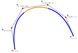
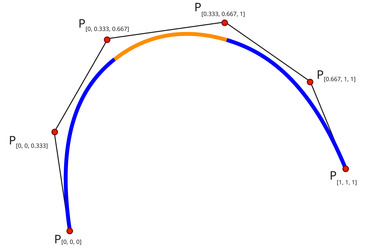
English: This curve is a cubic parametric polynomial spline composed of three segments and may be called a degree three, or, alternatively, an order four spline curve. The position of each point on the curve stems from one in a set of three polynomial parametric functions fi(u). The four terms of each polynomial consist of coefficients of geometric points scaled (or weighted) by basis functions expressed in terms of the parameter u. The geometric points constitute an ordered set and form the control mesh around the curve. The polynomials essentially sample each of four consecutive points from the mesh by weighting factors, these computed by the basis functions for particular values of u. The sum of these weighted positions plot a point on the curve for the corresponding values of u. Each point on the curve is a particular barycentric combination of a set of four consecutive points from the mesh, where the term 'barycentric combination' infers that the weights produced by the basis functions add up to one (partition unity), a necessary condition for coordinate-independent calculations. In a general setting of arbitrary weights, the weighted sums of geometric points that have just been described would also incorporate the distances between each point and the origin of the coordinate system and the shape of the curve would change as the mesh of points moves. With weights that partition unity, the distance of points from the origin can be factored away and the shape of the curve would depend only on the relative positions of the points comprising the mesh. The term 'control point' can be applied to the elements of the mesh because moving a control point changes the positional information that is being blended into the curve, thereby changing its shape.
For splines, knot sequences determine which of the polynomial parametric functions plot the curve. Knot sequences are ordered pairs of parametric values and an associated multiplicity that signal a change in the control points used as geometric coefficients. Consider a four control point wide 'selection box'; its position along a linear arrangement of control points depends on the highest value knot that is still less than or equal to the value of parameter u. The control point that is to be utilized as the first coefficient in the parametric polynomial is selected by the sum of multiplicities of all knots less than or equal to u, minus the order of the curve. One can imagine the selection box shifting over one or more control points as u traverses its parametric range. In this example, there are single multiplicity knots at the parametric values of 1/3 and 2/3. The first four control points fully dictate the shape of the leftmost blue segment of the curve; they prevail for parametric values less than 1/3. For parametric values equal to or greater than 1/3, the middle four control points plot the curve, shown here as an orange segment. For the third segment of the curve, plotted with parametric values of 2/3 or greater, the rightmost four control points shape the curve. In this example, multiplicity four knots resided at either end of the curve and ensures that the curve is defined over the entire parametric range of u and that the curve interpolates its end points. This is not a general case; intervals can be partitioned by single multiplicity knots over the entire parametric range. There will necessarily be intervals on either end of the parametric range where the curve is not defined. The index positioning the selection box is either too far to the left or right so that there are an insufficient number of control points available to blend into the curve; the curve is undefined for those intervals. There is a connection between knot multiplicity and curve continuity. Roughly, higher multiplicity knots induce a greater change in the number of control points used when plotting from one segment to the next, so a follow on segment is 'less like' its predecessor for higher multiplicity knots. For cubic curves, a multiplicity two knot implies continuity only up to the first derivative; the second derivative will jump in value from one segment to the next. For multiplicity three knots, only positional continuity is obtained; the curve may exhibit a sharp corner because there can be a jump in the first derivative of the curve. In this diagram, the control point indices happen to be in blossom format because there is an association between control points and knot sub-sequences. It is beyond the scope of this brief caption to detail this association; suffice to say that, among other matters, it is a particular way to label control points that happen to demarcate parametric regions where the control point has its greatest weight or "influence." Readers wishing to know more about the association between control points and knot sub-sequences should consult Chapter 6, "Blossoming" of Ron Goldman's Pyramid Algorithms 2003, Morgan Kaufman Publishers. ISBN 1-55860-354-9 |
| Date | |
| Source | Travail personnel |
| Auteur | Garry R. Osgood |
Conditions d’utilisation
- Vous êtes libre :
- de partager – de copier, distribuer et transmettre cette œuvre
- d’adapter – de modifier cette œuvre
- Sous les conditions suivantes :
- paternité – Vous devez donner les informations appropriées concernant l'auteur, fournir un lien vers la licence et indiquer si des modifications ont été faites. Vous pouvez faire cela par tout moyen raisonnable, mais en aucune façon suggérant que l’auteur vous soutient ou approuve l’utilisation que vous en faites.
- partage à l’identique – Si vous modifiez, transformez, ou vous basez sur cette œuvre, vous devez distribuer votre contribution sous la même licence ou une licence compatible avec celle de l’original.

|
Vous avez la permission de copier, distribuer et modifier ce document selon les termes de la GNU Free Documentation License version 1.2 ou toute version ultérieure publiée par la Free Software Foundation, sans sections inaltérables, sans texte de première page de couverture et sans texte de dernière page de couverture. Un exemplaire de la licence est inclus dans la section intitulée GNU Free Documentation License. |
Historique du fichier
Cliquer sur une date et heure pour voir le fichier tel qu'il était à ce moment-là.
| Date et heure | Vignette | Dimensions | Utilisateur | Commentaire | |
|---|---|---|---|---|---|
| actuel | 12 octobre 2017 à 16:37 | | 780 × 532 (10 kio) | Nicoguaro | Remove background and change unnecessary paths to objects. |
| 4 juillet 2008 à 20:19 |  | 780 × 532 (131 kio) | Garry R. Osgood | {{Information |Description= |Source= |Date= |Author= |Permission= |other_versions= }} Category:Splines | |
| 3 juillet 2008 à 01:13 |  | 780 × 532 (130 kio) | Garry R. Osgood | {{Information |Description={{en|1=This curve is a cubic parametic polynomial spline comprised of three segments. That is, the [''x'', ''y''] coordinates of each point on the curve stem from a pair of functions ''f<sub>x</sub>(u) |
Utilisation du fichier
La page suivante utilise ce fichier :
Usage global du fichier
Les autres wikis suivants utilisent ce fichier :
- Utilisation sur bg.wikipedia.org
- Utilisation sur en.wikipedia.org
- Utilisation sur et.wikipedia.org
- Utilisation sur fa.wikipedia.org
- Utilisation sur mk.wikipedia.org
- Utilisation sur uk.wikipedia.org
- Utilisation sur zh.wikipedia.org