
Fichier:Karmarkar.svg

Taille de cet aperçu PNG pour ce fichier SVG : 720 × 540 pixels. Autres résolutions : 320 × 240 pixels | 640 × 480 pixels | 1 024 × 768 pixels | 1 280 × 960 pixels | 2 560 × 1 920 pixels.
Fichier d’origine (Fichier SVG, nominalement de 720 × 540 pixels, taille : 43 kio)
Ce fichier et sa description proviennent de Wikimedia Commons.
Description
| Description |
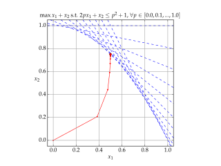
English: Solution of example LP in Karmarkar's algorithm.
Blue lines show the constraints, Red shows each iteration of the algorithm. |
| Date | |
| Source | Travail personnel |
| Auteur | Gjacquenot |
Conditions d’utilisation
Moi, en tant que détenteur des droits d’auteur sur cette œuvre, je la publie sous la licence suivante :
Ce fichier est sous la licence Creative Commons Attribution – Partage dans les Mêmes Conditions 4.0 International.
- Vous êtes libre :
- de partager – de copier, distribuer et transmettre cette œuvre
- d’adapter – de modifier cette œuvre
- Sous les conditions suivantes :
- paternité – Vous devez donner les informations appropriées concernant l'auteur, fournir un lien vers la licence et indiquer si des modifications ont été faites. Vous pouvez faire cela par tout moyen raisonnable, mais en aucune façon suggérant que l’auteur vous soutient ou approuve l’utilisation que vous en faites.
- partage à l’identique – Si vous modifiez, transformez, ou vous basez sur cette œuvre, vous devez distribuer votre contribution sous la même licence ou une licence compatible avec celle de l’original.
Source code (Python)
#!/usr/bin/env python
# -*- coding: utf-8 -*-
#
# Python script to illustrate the convergence of Karmarkar's algorithm on
# a linear programming problem.
#
# http://en.wikipedia.org/wiki/Karmarkar%27s_algorithm
#
# Karmarkar's algorithm is an algorithm introduced by Narendra Karmarkar in 1984
# for solving linear programming problems. It was the first reasonably efficient
# algorithm that solves these problems in polynomial time.
#
# Karmarkar's algorithm falls within the class of interior point methods: the
# current guess for the solution does not follow the boundary of the feasible
# set as in the simplex method, but it moves through the interior of the feasible
# region, improving the approximation of the optimal solution by a definite
# fraction with every iteration, and converging to an optimal solution with
# rational data.
#
# Guillaume Jacquenot
# 2015-05-03
# CC-BY-SA

import numpy as np
import matplotlib
from matplotlib.pyplot import figure, show, rc, grid

class ProblemInstance():
    def __init__(self):
        n = 2
        m = 11
        self.A = np.zeros((m,n))
        self.B = np.zeros((m,1))
        self.C = np.array([[1],[1]])
        self.A[:,1] = 1
        for i in range(11):
            p = 0.1*i
            self.A[i,0] = 2.0*p
            self.B[i,0] = p*p + 1.0

class KarmarkarAlgorithm():
    def __init__(self,A,B,C):
        self.maxIterations = 100
        self.A = np.copy(A)
        self.B = np.copy(B)
        self.C = np.copy(C)
        self.n = len(C)
        self.m = len(B)
        self.AT = A.transpose()
        self.XT = None

    def isConvergeCriteronSatisfied(self, epsilon = 1e-8):
        if np.size(self.XT,1)<2:
            return False
        if np.linalg.norm(self.XT[:,-1]-self.XT[:,-2],2) < epsilon:
            return True

    def solve(self, X0=None):
        # No check is made for unbounded problem
        if X0 is None:
            X0 = np.zeros((self.n,1))
        k = 0
        X = np.copy(X0)
        self.XT = np.copy(X0)
        gamma = 0.5
        for _ in range(self.maxIterations):
            if self.isConvergeCriteronSatisfied():
                break
            V = self.B-np.dot(self.A,X)
            VM2 = np.linalg.matrix_power(np.diagflat(V),-2)
            hx = np.dot(np.linalg.matrix_power(np.dot(np.dot(self.AT,VM2),self.A),-1),self.C)
            hv = -np.dot(self.A,hx)
            coeff = np.infty
            for p in range(self.m):
                if hv[p,0]<0:
                    coeff = np.min((coeff,-V[p,0]/hv[p,0]))
            alpha = gamma * coeff
            X += alpha*hx
            self.XT = np.concatenate((self.XT,X),axis=1)

    def makePlot(self,outputFilename = r'Karmarkar.svg', xs=-0.05, xe=+1.05):
        rc('grid', linewidth = 1, linestyle = '-', color = '#a0a0a0')
        rc('xtick', labelsize = 15)
        rc('ytick', labelsize = 15)
        rc('font',**{'family':'serif','serif':['Palatino'],'size':15})
        rc('text', usetex=True)

        fig = figure()
        ax = fig.add_axes([0.12, 0.12, 0.76, 0.76])
        grid(True)
        ylimMin = -0.05
        ylimMax = +1.05
        xsOri = xs
        xeOri = xe
        for i in range(np.size(self.A,0)):
            xs = xsOri
            xe = xeOri
            a = -self.A[i,0]/self.A[i,1]
            b = +self.B[i,0]/self.A[i,1]
            ys = a*xs+b
            ye = a*xe+b
            if ys>ylimMax:
                ys = ylimMax
                xs = (ylimMax-b)/a
            if ye<ylimMin:
                ye = ylimMin
                xe = (ylimMin-b)/a
            ax.plot([xs,xe], [ys,ye], \
                    lw = 1, ls = '--', color = 'b')
        ax.set_xlim((xs,xe))
        ax.plot(self.XT[0,:], self.XT[1,:], \
                lw = 1, ls = '-', color = 'r', marker = '.')
        ax.plot(self.XT[0,-1], self.XT[1,-1], \
                lw = 1, ls = '-', color = 'r', marker = 'o')
        ax.set_xlim((ylimMin,ylimMax))
        ax.set_ylim((ylimMin,ylimMax))
        ax.set_aspect('equal')
        ax.set_xlabel('$x_1$',rotation = 0)
        ax.set_ylabel('$x_2$',rotation = 0)
        ax.set_title(r'$\max x_1+x_2\textrm{ s.t. }2px_1+x_2\le p^2+1\textrm{, }\forall p \in [0.0,0.1,...,1.0]$',
                     fontsize=15)
        fig.savefig(outputFilename)
        fig.show()

if __name__ == "__main__":
    p = ProblemInstance()
    k = KarmarkarAlgorithm(p.A,p.B,p.C)
    k.solve(X0 = np.zeros((2,1)))
    k.makePlot(outputFilename = r'Karmarkar.svg', xs=-0.05, xe=+1.05)
Historique du fichier
Cliquer sur une date et heure pour voir le fichier tel qu'il était à ce moment-là.
| Date et heure | Vignette | Dimensions | Utilisateur | Commentaire | |
|---|---|---|---|---|---|
| actuel | 22 novembre 2017 à 17:34 | | 720 × 540 (43 kio) | DutchCanadian | The right hand side for the constraints appears to be p<sup>2</sup>+1, rather than p<sup>2</sup>, going by both the plot and the code (note the line <tt>self.B[i,0] = p*p + 1.0</tt>). Updated the header line. |
| 3 mai 2015 à 21:29 |  | 720 × 540 (41 kio) | Gjacquenot | Updated constraint display | |
| 3 mai 2015 à 21:26 |  | 720 × 540 (41 kio) | Gjacquenot | Updated constraint display | |
| 3 mai 2015 à 21:17 |  | 720 × 540 (41 kio) | Gjacquenot | Updated constraint display | |
| 3 mai 2015 à 20:54 |  | 720 × 540 (41 kio) | Gjacquenot | User created page with UploadWizard |
Utilisation du fichier
La page suivante utilise ce fichier :
Usage global du fichier
Les autres wikis suivants utilisent ce fichier :
- Utilisation sur ar.wikipedia.org
- Utilisation sur en.wikipedia.org
- Utilisation sur ja.wikipedia.org
- Utilisation sur ko.wikipedia.org
- Utilisation sur pt.wikipedia.org
- Utilisation sur ru.wikipedia.org
- Utilisation sur simple.wikipedia.org
- Utilisation sur uk.wikipedia.org
- Utilisation sur zh.wikipedia.org